Common Networks

CNN (MNIST)

Setup

from tensorflow.examples.tutorials.mnist import input_data
import tensorflow as tf
import numpy as np
import matplotlib.pyplot as plt

tf.set_random_seed(1)
np.random.seed(1)

1
2
3
4
5
6
7

Prepare Input

BATCH_SIZE = 50
LR = 0.001  # learning rate

mnist = input_data.read_data_sets('./mnist', one_hot=True)
test_x = mnist.test.images[:2000] # use only 2000 images for testing
test_y = mnist.test.labels[:2000]

tf_x = tf.placeholder(tf.float32, [None, 28*28]) 
tf_y = tf.placeholder(tf.int32, [None, 10])
tf_x /= 255. # normalize image pixels (pixels' max value is 255)

# (batch, height, width, channel)
images = tf.reshape(tf_x, [-1, 28, 28, 1])

1
2
3
4
5
6
7
8
9
10
11
12
13

CNN

conv1 = tf.layers.conv2d(   # shape (28, 28, 1)
    inputs=images,
    filters=16,
    kernel_size=5,
    strides=1,
    padding='same',
    activation=tf.nn.relu
) # -> (28, 28, 16)
pool1 = tf.layers.max_pooling2d(
    conv1,
    pool_size=2,
    strides=2,
) # -> (14, 14, 16)
conv2 = tf.layers.conv2d(pool1, 32, 5, 1, 'same',
                         activation=tf.nn.relu) # -> (14, 14, 32)
pool2 = tf.layers.max_pooling2d(conv2, 2, 2)    # -> (7, 7, 32)
flat = tf.reshape(pool2, [-1, 7*7*32])          # -> (7*7*32, )
output = tf.layers.dense(flat, 10)              # output layer

1
2
3
4
5
6
7
8
9
10
11
12
13
14
15
16
17
18

Loss / Training Ops

loss = tf.losses.softmax_cross_entropy(onehot_labels=tf_y, logits=output)
train_op = tf.train.AdamOptimizer(LR).minimize(loss)
accuracy = tf.metrics.accuracy(labels=tf.argmax(tf_y, axis=1), 
                               predictions=tf.argmax(output, axis=1))[1]

1
2
3
4

Training

sess = tf.Session()
init_op = tf.group(tf.global_variables_initializer(), 
                   tf.local_variables_initializer())
sess.run(init_op)

for step in range(600):
    b_x, b_y = mnist.train.next_batch(BATCH_SIZE)
    _, loss_ = sess.run([train_op, loss], {tf_x: b_x, tf_y: b_y})

    if step % 50 == 0:
        accuracy_ = sess.run(accuracy, {tf_x: test_x, tf_y: test_y})
        print('Step:', step, '| train loss: %.4f' %
              loss_, '| test accuracy: %.2f' % accuracy_)

1
2
3
4
5
6
7
8
9
10
11
12
13

Testing

# print 10 predictions from test data
test_output = sess.run(output, {tf_x: test_x[:10]})
pred_y = np.argmax(test_output, 1)
print(pred_y, 'prediction number')
print(np.argmax(test_y[:10], 1), 'real number') # test_y is one-hot encoded

1
2
3
4
5

RNN Classification (MNIST)

Setup (skip, same as CNN)

Prepare Input

# Hyper Parameters
BATCH_SIZE = 64
TIME_STEP = 28          # rnn time step / image height
INPUT_SIZE = 28         # rnn input size / image width
LR = 0.01               # learning rate

mnist = input_data.read_data_sets('./mnist', one_hot=True)
test_x = mnist.test.images[:2000]
test_y = mnist.test.labels[:2000]

# shape(batch, 784)
tf_x = tf.placeholder(tf.float32, [None, TIME_STEP * INPUT_SIZE])
tf_y = tf.placeholder(tf.int32, [None, 10])

# (batch, height, width, channel)
image = tf.reshape(tf_x, [-1, TIME_STEP, INPUT_SIZE])

1
2
3
4
5
6
7
8
9
10
11
12
13
14
15
16

RNN

rnn_cell = tf.nn.rnn_cell.LSTMCell(num_units=64)
outputs, (h_c, h_n) = tf.nn.dynamic_rnn(
    rnn_cell,                   # cell you have chosen
    image,                      # input
    initial_state=None,         # the initial hidden state
    dtype=tf.float32,           # must given if set initial_state = None
    # False: (batch, time step, input); True: (time step, batch, input)
    time_major=False,
)
# output based on the last output step
output = tf.layers.dense(outputs[:, -1, :], 10)

1
2
3
4
5
6
7
8
9
10
11

Loss / Training Ops (skip, same as CNN)

Training (skip, same as CNN)

Testing (skip, same as CNN)

[SideNote] Multi-layer RNN Cell

# create 2 LSTMCells
rnn_layers = [
    tf.nn.rnn_cell.LSTMCell(128),
    tf.nn.rnn_cell.LSTMCell(256)
]

# create a RNN cell composed sequentially of a number of RNNCells
multi_rnn_cell = tf.nn.rnn_cell.MultiRNNCell(rnn_layers)

# 'outputs' is a tensor of shape [batch_size, max_time, 256]
# 'state' is a N-tuple where N is the number of LSTMCells containing a
# tf.contrib.rnn.LSTMStateTuple for each cell
outputs, state = tf.nn.dynamic_rnn(cell=multi_rnn_cell,
                                   inputs=data,
                                   dtype=tf.float32)

1
2
3
4
5
6
7
8
9
10
11
12
13
14
15

RNN Regression (Seq-to-Seq)

Setup

import tensorflow as tf
import numpy as np
import matplotlib.pyplot as plt

1
2
3

Prepare Input

TIME_STEP = 10       # rnn time step
INPUT_SIZE = 1      # rnn input size
CELL_SIZE = 32      # rnn cell size
LR = 0.02           # learning rate

# Generate sin wave as input and cos wave as target
steps = np.linspace(0, np.pi*2, 100, dtype=np.float32)
x_np = np.sin(steps)
y_np = np.cos(steps)

tf_x = tf.placeholder(tf.float32, [None, TIME_STEP, INPUT_SIZE])
tf_y = tf.placeholder(tf.float32, [None, TIME_STEP, INPUT_SIZE])

1
2
3
4
5
6
7
8
9
10
11
12

RNN

rnn_cell = tf.nn.rnn_cell.LSTMCell(num_units=CELL_SIZE)
# very first hidden state
init_s = rnn_cell.zero_state(batch_size=1, dtype=tf.float32)
outputs, final_s = tf.nn.dynamic_rnn(
    rnn_cell,                   # cell you have chosen
    tf_x,                       # input
    initial_state=init_s,       # the initial hidden state
   
    # False: (batch, time step, input)
    # True:  (time step, batch, input)
    time_major=False,
)
# reshape 3D output to 2D (flattened) for fully connected layer
outs2D = tf.reshape(outputs, [-1, CELL_SIZE])
net_outs2D = tf.layers.dense(outs2D, INPUT_SIZE)
# reshape back to 3D
outs = tf.reshape(net_outs2D, [-1, TIME_STEP, INPUT_SIZE])

1
2
3
4
5
6
7
8
9
10
11
12
13
14
15
16
17

Loss / Training Ops

loss = tf.losses.mean_squared_error(labels=tf_y, predictions=outs)
train_op = tf.train.AdamOptimizer(LR).minimize(loss)

1
2

Training

sess = tf.Session()
sess.run(tf.global_variables_initializer())

for step in range(160):
    start, end = step * np.pi, (step+1)*np.pi   # time range
    # use sin predicts cos
    steps = np.linspace(start, end, TIME_STEP)
    # shape (batch, time_step, input_size)
    x = np.sin(steps)[np.newaxis, :, np.newaxis]
    y = np.cos(steps)[np.newaxis, :, np.newaxis]
    
    if 'final_s_' not in globals(): # first state, no any hidden state
        feed_dict = {tf_x: x, tf_y: y}
    else:                           # has hidden state, so pass it to rnn
        feed_dict = {tf_x: x, tf_y: y, init_s: final_s_}
    
    _, pred_, final_s_ = sess.run(
        [train_op, outs, final_s], feed_dict)     # train

    # plotting
    plt.plot(steps, y.flatten(), 'r-')
    plt.plot(steps, pred_.flatten(), 'b-')
    plt.ylim((-1.2, 1.2))
    plt.draw()
    plt.pause(0.05)

1
2
3
4
5
6
7
8
9
10
11
12
13
14
15
16
17
18
19
20
21
22
23
24
25

AutoEncoder (MNIST)

Setup (skip, same as CNN)

Prepare Input

BATCH_SIZE = 64
LR = 0.002  # learning rate
N_TEST_IMG = 5

# use not one-hotted target data
mnist = input_data.read_data_sets('./mnist', one_hot=False)
test_x = mnist.test.images[:200]
test_y = mnist.test.labels[:200]

tf_x = tf.placeholder(tf.float32, [None, 28*28])

1
2
3
4
5
6
7
8
9
10

Encoder

en0 = tf.layers.dense(tf_x, 128, tf.nn.tanh)
en1 = tf.layers.dense(en0, 64, tf.nn.tanh)
en2 = tf.layers.dense(en1, 12, tf.nn.tanh)
encoded = tf.layers.dense(en2, 3)

1
2
3
4

Decoder

de0 = tf.layers.dense(encoded, 12, tf.nn.tanh)
de1 = tf.layers.dense(de0, 64, tf.nn.tanh)
de2 = tf.layers.dense(de1, 128, tf.nn.tanh)
decoded = tf.layers.dense(de2, 28*28, tf.nn.sigmoid)

1
2
3
4

Loss / Training Ops

loss = tf.losses.mean_squared_error(labels=tf_x, predictions=decoded)
train = tf.train.AdamOptimizer(LR).minimize(loss)

1
2

Setup subplots for visualizing training progress

f, a = plt.subplots(2, N_TEST_IMG, figsize=(5, 2))
plt.ion()   # continuous plotting

# Plot first N test images during trainig
test_data = mnist.test.images[:N_TEST_IMG]
for i in range(N_TEST_IMG):
    a[0][i].imshow(np.reshape(test_data[i], (28, 28)), cmap='gray')
    a[0][i].set_xticks(())
    a[0][i].set_yticks(())

1
2
3
4
5
6
7
8
9

Training

sess = tf.Session()
sess.run(tf.global_variables_initializer())

for step in range(8000):
    b_x, b_y = mnist.train.next_batch(BATCH_SIZE)
    _, encoded_, decoded_, loss_ = sess.run(
        [train, encoded, decoded, loss], {tf_x: b_x})

    if step % 100 == 0: # plotting
        print('train loss: %.4f' % loss_)
        # plotting decoded image (second row)
        decoded_data = sess.run(decoded, {tf_x: test_data})
        for i in range(N_TEST_IMG):
            a[1][i].clear()
            a[1][i].imshow(np.reshape(decoded_data[i], (28, 28)), cmap='gray')
            a[1][i].set_xticks(())
            a[1][i].set_yticks(())
        plt.draw()
        plt.pause(0.01)
plt.ioff()

1
2
3
4
5
6
7
8
9
10
11
12
13
14
15
16
17
18
19
20

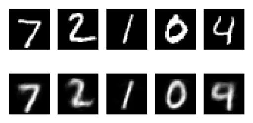
First row is the original test images, second row is 'decoded' test images.

Test data 3D visualization

from mpl_toolkits.mplot3d import Axes3D
from matplotlib import cm

fig = plt.figure(2)
ax = Axes3D(fig)
X, Y, Z = encoded_data[:, 0], encoded_data[:, 1], encoded_data[:, 2]

test_data = test_x[:200]
encoded_data = sess.run(encoded, {tf_x: test_data})

for x, y, z, s in zip(X, Y, Z, test_y):
    c = cm.rainbow(int(255*s/9))
    ax.text(x, y, z, s, backgroundcolor=c)
    
ax.set_xlim(X.min(), X.max())
ax.set_ylim(Y.min(), Y.max())
ax.set_zlim(Z.min(), Z.max())
plt.show()

1
2
3
4
5
6
7
8
9
10
11
12
13
14
15
16
17
18

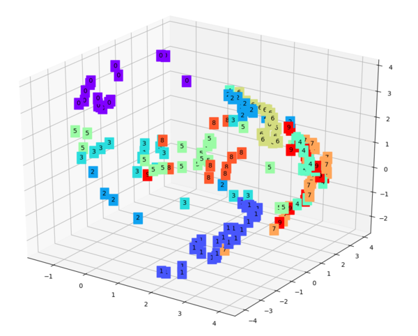
Visualize relationships between digits that encoder has learned. Use t-SNE for dimension reduction.

Common Networks

# CNN (MNIST)

# RNN Classification (MNIST)

# RNN Regression (Seq-to-Seq)

# AutoEncoder (MNIST)

CNN (MNIST)

RNN Classification (MNIST)

RNN Regression (Seq-to-Seq)

AutoEncoder (MNIST)